Chapter 4 Correlations
Correlation is a measure of the strength and direction of association that exists between two variables. Correlation coefficients (\(r\)) assume values in the range from −1 to +1, where ±1 indicates the strongest possible positive or negative correlation and 0 indicates no linear association between the variables.
4.1 Pearson correlation
We start by looking at the Pearson correlation coefficient. Here we compare the built-in test (in R) for the Pearson correlation with the equivalent linear model.
The equivalent linear model is the basic regression of \(y\) on \(x\), specified as follows: \(y = \beta_0 + \beta_1x \qquad H_0: \beta_1 = 0\)
The two tests are written using the following R code:
# Pearson (built-in test)
cor.test(y, x, method = "pearson")
# Linear model
lm(y ~ 1 + x) %>% summary() %>% print(digits = 8)
If you were to run the code above, you would see the following the key statistics found in the output of each test:
| Test | r | slope | t | p-value |
|---|---|---|---|---|
| cor.test (Pearson) | -0.2318 | -1.6507 | 0.1053 | |
| lm | -0.4636 | -1.6507 | 0.1053 |
The output shows that the correlation coefficient (\(r\)) has a p-value of 0.1053, which is exactly the same as the p-value for the slope of the linear model. In this case, we would not reject the null hypothesis that there was no correlation between the two variables (at the 0.05 level of significance).
The main difference is that the linear model returns the slope of the relationship, \(\beta_1\) (which in this case is -0.4636), rather than the correlation coefficient, \(r\). The slope is usually much more interpretable and informative than the correlation coefficient.
Additional note (optional):
It may be useful to understand how the Pearson correlation coefficient (\(r\)) and the regression coefficient or slope (\(\beta_1\)) are related, which is by the following formula:
\(\beta_1 = r \cdot sd_y / sd_x\)
This shows that:
- When both
xandyhave the same standard deviations (\(sd_x\) and \(sd_y\)) then the slope (\(\beta_1\)) will be equal to the correlation coefficient (\(r\)) - The ratio of the slope to the correlation coefficient (\(\beta_1 / r\)) is equal to the ratio of the standard deviations (\(sd_y / sd_x\)). In this example, the standard deviation of
yis exactly twice as large asx, which is why the slope has twice the magnitude of the correlation coefficient. - The slope from the linear model will always have the same sign (+ or -) as the correlation coefficient (as standard deviations are always positive).
4.2 Spearman correlation
There will be times when it is more appropriate to use the Spearman rank correlation than the Pearson correlation. This could be the case when:
- The relationship between the variables is not linear, i.e. not a straight line;
- The data is not normally distributed;2
- The data has large outliers; or
- When you are working with ordinal rather than continuous data.3
The Spearman correlation is a non-parameteric test as it does not require that the parameters of the linear model hold true. For example, there does not need to be a linear relationship between the two variables, and the data does not need to be normally distributed.
The Spearman rank correlation is the same as a Pearson correlation but using the rank of the values in our samples. This is an approximation only, which Lindeløv shows is approximate when the sample size is greater than 10 and almost perfect when the sample is greater than 20.
This is also the same as the linear model using rank-transformed values of \(x\) and \(y\):
\(rank(y) = \beta_0 + \beta_1 \cdot rank(x) \qquad H_0: \beta_1 = 0\)
For a comparison of the Spearman test, the Pearson test (using ranks) and the linear model (also using ranks) we run the following code:
# Spearman
cor.test(y, x, method = "spearman")

# Pearson using ranks
cor.test(rank(y), rank(x), method = "pearson")

# Linear model using rank
lm <- lm(rank(y) ~ 1 + rank(x))
  lm %>% summary() %>% print(digits = 5) # show summary ouput
The output of this code is as follows:
| Test | correlation | slope | p.value |
|---|---|---|---|
| cor.test (Spearman) | -0.2266 | 0.1135 | |
| cor.test (Pearson with ranks) | -0.2266 | 0.1135 | |
| lm (with ranks) | -0.2266 | 0.1135 |
This shows that the results are all the same (or at least very close approximations). When ranks are used, the slope of the linear model (\(\beta_1\)) has the same value as the correlation coefficient (\(r\)). Note that the slope from the linear model has an intuitive interpretation, which is the number of ranks \(y\) changes for each change in rank of \(x\).
Given the similarity of these tests, Lindeløv notes that:
One interesting implication is that many “non-parametric tests” are about as parametric as their parametric counterparts with means, standard deviations, homogeneity of variance, etc. - just on rank-transformed data.
Finally, the figure below (reproduced from the original book) illustrates how the Pearson and Spearman correlations are equivalent to linear models, with the latter being based on rank-transformed values.
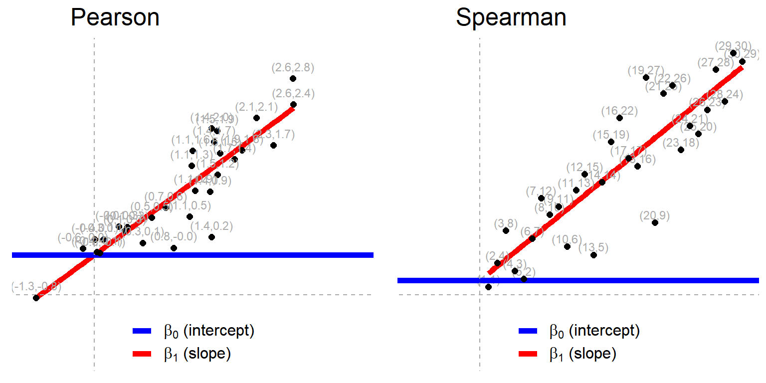
Figure 4.1: Pearson and Spearman correlations as linear models
Technically the variables should have bivariate normality, which means they are normally distributed when added together, but this is complex and so it is common just to assess whether the variables are individually normal (explained here on the Laerd website). If bi-variate normality does not hold then you will still get a fair estimate of \(r\), but the inferential tests (t-statistics and p-values) could be misleading (explained here).↩
see Chapter 9 for a description of the different types of data.↩