Chapter 6 Two means (independent samples)
These tests compare the means of two independent or unrelated groups, in order to determine whether there is statistical evidence that the population means are significantly different. Examples include:
- Do first year graduate salaries differ based on gender? and
- Is there is a difference in test anxiety based on educational level (undergraduate vs postgraduate)?
A key question is whether or not the variances of the two samples being tested are equal.4 In general terms:
- If the samples have equal variance then an independent-sample t-test (Student’s t-test) could be used.
- If the samples have unequal variance then the Welch’s t-test can be used, as this does not assume identical variances.
- If the samples are not normally distibuted, or if the other requirements of the above tests are not met, then the non-parametric Mann-Whitney U test could be used.
This is somewhat simplistic, and the choice of tests is not always clear (see the discussion here on StackExchange for example). The following sections goes through each of these tests in turn, and describes how they can be approximated by an equivalent linear model.
6.1 Independent t-test
The independent t-test can be used to compare the means of two unrelated groups. Assumptions include:
- Independence of observations (independent samples / groups);
- Normal distribution (approximately) of the dependent variable for each group, though this might not be an issue for large samples;
- No outliers; and
- Homogeneity of variances; i.e. variances are approximately equal across the two groups.
Student’s t-test:
In R, we can assesses the difference between two groups using the t.test. This has the default assumptions that the two samples are not paired, and that their variances are not equal.
Equivalent linear model:
The equivalent linear model uses a dummy variable to represent the two groups (see the explanation of dummy variables explained by Lindeløv in section 5.1.3 of the original book).
The linear model takes the form:
\(y = \beta_0 + \beta_1 \cdot x_i \qquad H_0: \beta_0 = 0\)
where \(x_i\) is a dummy variable taking the value of 0 or 1, indicating whether observation \(i\) is from the reference group (0) or the other group (1). For example, \(y\) could be a measure of income and \(x_i\) could be a dummy variable taking the value of 0 for women and 1 for men.
The use of dummy variables is illustrated below. The intercept (\(\beta_0\)) is the sample average for observations in our reference group (in this example, women) when \(x = 0\). The slope (\(\beta_1\)) is the difference in the averages of the two groups. In this example, when \(x = 1\) (indicating men), the average salary is equal to \(\beta_0 + \beta_1\). Therefore, \(\beta_1\) is the difference between the two groups, and we want to assess whether this difference is significantly different from zero.
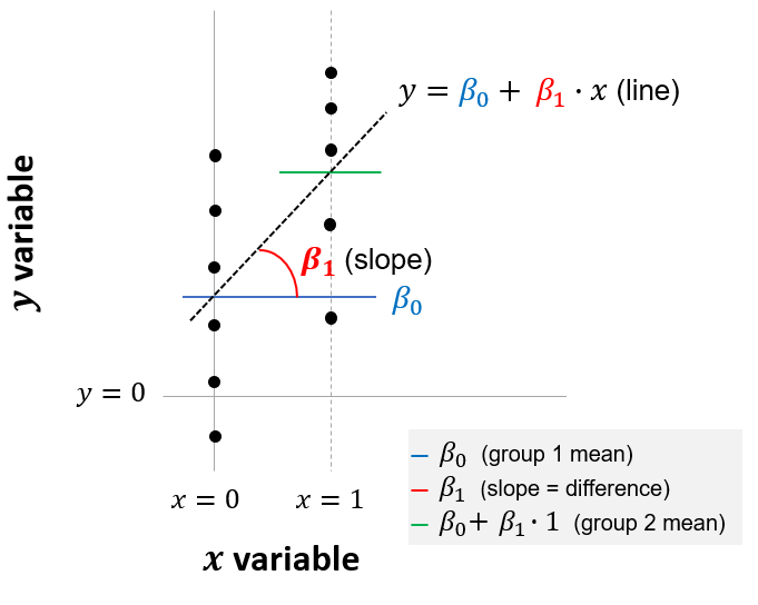
Figure 6.1: Linear model equivalent to independent-sample t-test
Comparison:
Let’s say we want to compare the means of two groups in our example dataset, y and y2.
We start by creating a dummy variable to represent the two groups. The new variable is called group_y2 and takes a value of 0 for observations in group y and a value of 1 for observations in group y2. This is done using the following code:
Here’s a sample of six rows from our new data set, which now includes the dummy variable:
| group | value | group_y2 |
|---|---|---|
| y | 1.1535602 | 0 |
| y | 1.1881680 | 0 |
| y | -1.3557817 | 0 |
| y2 | 0.1030347 | 1 |
| y2 | -0.2808907 | 1 |
| y2 | 0.6238886 | 1 |
Now we’ve organized our data, we can compare the results of the built-in independent t-test with the linear model:
# independent t-test (built-in test)
t.test(y2, y, var.equal = TRUE)
  # default is mu = 0, i.e. the null hypothesis that the difference in means is zero

# Linear model
lm <- lm(value ~ 1 + group_y2, data = mydata_dummy)
  lm %>% summary() %>% print(digits = 8) # show summary output
  confint(lm) # show confidence intervals
The outputs from the independent t-test and the equivalent linear model are shown below. The t statistic, p-value and confidence intervals are identical. While the t-test reports the averages of the two samples, the linear model reports the average of the reference group (0.3 for y) and the difference between the average of this reference group and the other group indicated by the dummy variable (a difference of +0.2).
| Test | mean.y | mean.y2 | difference | t | p.value | conf.low | conf.high |
|---|---|---|---|---|---|---|---|
| t-test | 0.3 | 0.5 | 0.5657 | 0.5729 | -0.5016 | 0.9016 | |
| lm (with dummy) | 0.3 | 0.2 | 0.5657 | 0.5729 | -0.5016 | 0.9016 |
6.2 Welch’s t-test
If the two samples have unequal variance then Welch’s t-test could be used.
In fact, there is an argument that we should use Welch’s t-test by default, rather than the independent Student’s t-test, because Welch’s t-test performs better than the t-test whenever sample sizes and variances are unequal between groups, and gives the same result when sample sizes and variances are equal.
Welch’s t-test:
The Welch t-test is identical to the independent-sample Student’s t-test described above, except that it does not assume equal variance of the two samples. In R, we can use the built-in t.test. When entering the code, we just need to specify that the sample variances are not equal (though this is the default assumption anyway).
Equivalent linear model:
The equivalent linear model is based on generalized least squares (GLS). The GLS approach makes the assumption that there is a relationship between the variance of observations and one of the independent variables used in our regression (in this example, the gender dummy variable). In a GLS regression, less weight is given to the observations with a higher variance.
We don’t know the true relationship between variance and our independent variable(s) in the underlying population, so this relationship is estimated from our sample. The estimate is based on the relationship between residuals (i.e. observed values minus predicted values, based on an OLS regression) and an independent variable. Once we have estimated this relationship, we then re-weight each observation in our sample by dividing each observation by the predicted variance. The final GLS regression is then run on these re-weighted observations. A more detailed explanation of the GLS approach (without using matrix algebra!) can be found here.
In this example, when applying the GLS model in R, we specify that there is a different variance for group y and group y2.
Comparison:
The Welch’s t-test and the equivalent linear model are carried out as follows:
options(digits=10)
# t-test (built-in test)
t.test(y2, y, mu = 0, var.equal = FALSE, alternative = 'two.sided')
  # Note the assumption that variances are false

# Linear model (GLS)
lm <- nlme::gls(value ~ 1 + group_y2, weights = nlme::varIdent(form=~1|group), method="ML", data=mydata_dummy)
  lm %>% summary() %>% print(digits = 8) # show summary output
  confint(lm) # show confidence intervals
Here are the results, which are almost identical:
| Test | mean.y | mean.y2 | difference | t | p.value | conf.low | conf.high |
|---|---|---|---|---|---|---|---|
| t-test | 0.3 | 0.5 | 0.5657 | 0.5730 | -0.5023 | 0.9023 | |
| lm (GLS) | 0.3 | 0.2 | 0.5657 | 0.5729 | -0.4930 | 0.8930 |
Note that we get the same estimates for the means of \(y\) and \(y_2\) (of 0.3 and 0.5, respectively) from the t-test both with and without the assumption of equal variance. The unequal variance (heteroscedasticity) does not affect our estimates of the population means, but rather our assessment of whether or differences are statistically significant, in the form of t statistics, p-values and confidence intervals.
6.3 Mann-Whitney U test
If our usual assumptions don’t hold (e.g. normal distributions, or if we’re working with ordinal data) we can use a non-parametric version of these tests instead. When comparing two independent samples, this would be the Mann-Whitney U test.
Mann-Whitney U test:
This tests the null hypothesis that it is equally likely that a randomly selected value from one sample will be less than or greater than a randomly selected value from a second sample. In other words, if the null hypothesis was rejected, you would infer that values from one population are more likely to be higher or lower than values from another population.
The Man-Whitney U test is a Wilcoxon test but with two samples. It can be run using R’s built-in wilcox.test, this time with the (default) assumption that the observations are not paired.
Equivalent linear model:
Another way to describe the Mann-Whitney U test is as a test of mean ranks. It first ranks all your values for the dependent variable (e.g. income) from high to low, with the smallest rank assigned the smallest value. It then computes the mean rank in each group (e.g. male or female), and then computes the probability than random shuffling of those values between two groups would end up with the mean ranks as far apart as, or further apart, than you observed (see for example StackExchange and Laerd). If the resulting p-value was sufficiently small, you would infer that the difference in mean ranks between the samples was probably not due to chance, and that the values from one population were higher than those from another.
The equivalent linear model, with a close approximation, is a regression using the rank of the dependent variable:
\(rank(y_i) = \beta_0 + \beta_1 \cdot x_i \qquad H_0: \beta_0 = 0\)
where again \(x_i\) is a dummy variable indicating the group to which an observation belongs (in this example, 0 for women and 1 for men). Note that this uses the rank of the dependent variable, and not the signed rank as was the case with matched pairs.
Comparison:
Here is how you would run the Man-Whitney U test and equivalent linear model in R:
# Wilcoxon / Mann-Whitney U test (built-in)
wilcox.test(y, y2, paired = FALSE)

# Equivalent linear model
lm <- lm(rank(value) ~ 1 + group_y2, data = mydata_dummy)
  lm %>% summary() %>% print(digits = 8) # show summary output
The results are shown below. Both tests have very similar p-values. On this basis, we would not reject the null hypothesis that a value randomly selected from group y was not more likely to be higher or lower than one sampled from y2.
| Test | p-value | rank diff |
|---|---|---|
| wilcox.test | 0.7907 | |
| lm (ranks) | 0.7896 | 1.56 |
Digression - Mann-Whitney U test and medians:
It’s worth noting that, with additional assumptions, the Man-Whitney U test is also a test for different medians.
This requires the assumption that the two samples have an equal shape, and therefore an equal variance. Laerd illustrates this concept using the diagram below: on the left, the two samples (men and women) have the same shape, so the Mann-Whitney U test tests for differences in the median score for men and women. On the right, the samples have different shapes, so it is a more general test for whether a randomly-selected woman’s score is higher than a randomly-selected man’s score (without telling us anything about medians).
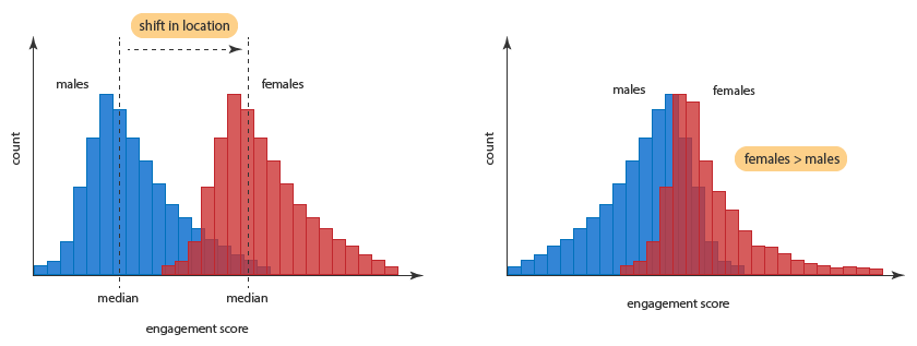
Figure 6.2: Man-Whitney U test and sample shapes
This can be tested with the Levene’s Test for Equality of Variances.↩