Chapter 3 The linear model
3.1 Overview of the linear model
The premise of this book is that many common statistical tests are really just special cases of the linear model.
This section provides an overview of the linear model. The description will be somewhat informal as it aims to provide an intuitive explanation rather than a rigorous technical description.
The linear model, or linear regression model, estimates the relationship between one continuous variable and one or more other variables. It is assumed that the relationship can be described as a straight line (hence the term ‘linear’).
For example, say we are looking at a variable \(y\) and we want to know its relationship with a variable \(x\). We assume that the relationship can be expressed as a mathematical relationship between \(y\) (the dependent, or response variable) and \(x\) (the explanatory variable):
\(y = \beta_0 + \beta_1 x\)
To illustrate what this equation is showing, imagine we have six observations of variables \(x\) and \(y\), which can be plotted as follows:
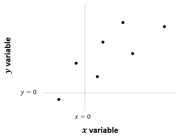
Figure 3.1: Six observations of x and y
We assume that this relationship can be represented by a straight line. The line is composed of an intercept (\(\beta_0\)) and a slope (\(\beta_1\)). Each point on this line represents our predicted value of \(y\) for a given value of \(x\).
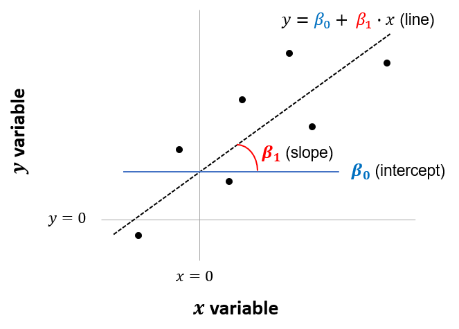
Figure 3.2: Intercept and slope of model
So how do we estimate the intercept and slope? In other words, how do we estimate what the values of \(\beta_0\) and \(\beta_1\) should be?
Linear regression estimates the line (i.e., slope and intercept) that minimizes the difference between our predicted values of \(y\) and the actual values of \(y\) that were observed in the original sample. These difference are referred to as “residuals”.
More specifically, linear regression minimizes the sum of the squared value of these residuals. So in the figure below, linear regression is used to estimate the line that would minimize the combined area of the purple squares. For this reason, the method is sometimes referred to as an “ordinary least squares” (OLS) regression.
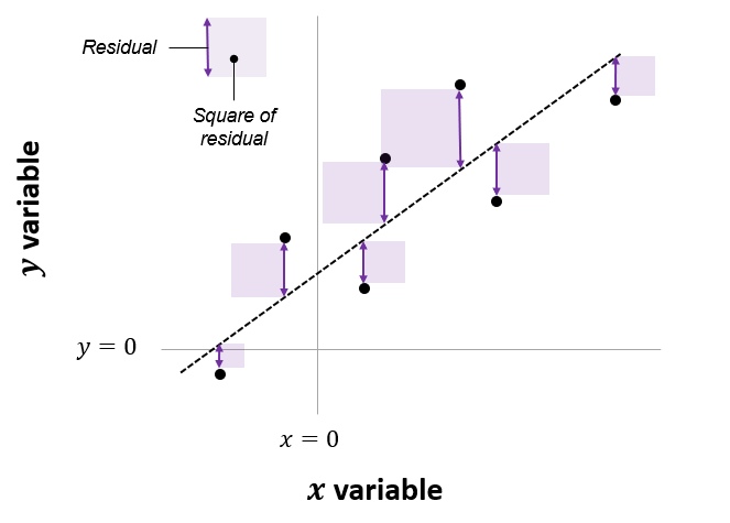
Figure 3.3: Line of best fit minimizes the sum of squared residuals
In the example above, we considered a dependent variable (\(y\)) that was being “explained” by one other variable, or predictor (\(x\)). But this can be expanded to include multiple predictors, for example with the model:
\(y = \beta_0 + \beta_1 x_1 + \beta_2 x_2 + \beta_3 x_3 ... + \beta_i x_i\)
This is referred to as multiple regression. In this case we still have only one intercept (\(\beta_0\)) but many slopes that need to be estimated (\(\beta_1\), \(\beta_2\) and so on). The same method can be used to estimate these parameters as was illustrated above, i.e. an OLS regression which minimizes the sum of squared residuals. This cannot be illustrated in a two-dimensional diagram, as was the case when a single predictor was used, but the exact same concept applies.
So that’s the linear model. The key premise of Lindeløv’s book many statistical tests are just special cases of this:
Everything below, from one-sample t-test to two-way ANOVA are just special cases of this system. Nothing more, nothing less.
3.2 Estimating linear models in R
To estimate linear models in R we use the lm() function.
For example, say we want to estimate the relationship between our sampled data for x and y. We will apply the following model: \(y = \beta_0 + \beta_1 x\)
In R, this can be written as follows:
lm(y ~ 1 + x) # Represents y = beta0 + beta1 * xIn the original book, the specified model is accompanied by the null hypothesis, \(H_0: \beta_1=0\). This is equivalent to saying that there is no relationship between x and y. The output from our linear model tells us whether there could be grounds for rejecting this null hypothesis of “no relationship”, in favor of the alternative hypothesis that there is a relationship.
A key output of interest, or test statistic, is the p-value.
- A small p-value (conventionally ≤ 0.05) indicates strong evidence against the null hypothesis, so you reject the null hypothesis of no relationship.1
- A larger p-value (> 0.05) indicates weak evidence against the null hypothesis, so you fail to reject the null hypothesis of no relationship.
Let’s see the output of the linear model for our sample data:
lm(y ~ 1 + x) %>% summary() %>% print(digits = 5) ##
## Call:
## lm(formula = y ~ 1 + x)
##
## Residuals:
## Min 1Q Median 3Q Max
## -3.33932 -1.65931 0.33492 1.36293 3.52139
##
## Coefficients:
## Estimate Std. Error t value Pr(>|t|)
## (Intercept) 0.30000 0.27799 1.0792 0.2859
## x -0.46355 0.28081 -1.6507 0.1053
##
## Residual standard error: 1.9657 on 48 degrees of freedom
## Multiple R-squared: 0.05372, Adjusted R-squared: 0.034006
## F-statistic: 2.725 on 1 and 48 DF, p-value: 0.10532As seen in the output above, \(\beta_1\) (the coefficient on x) has a p-value of 0.1053. This means we would fail to reject the null hypothesis that there was no relationship between x and y.
3.3 Assumptions
The inferences drawn from the linear model, as described above, are only valid if a number of assumptions hold. The following diagram, found in the book Broadening Your Statistical Horizons, can be used to explain these assumptions:
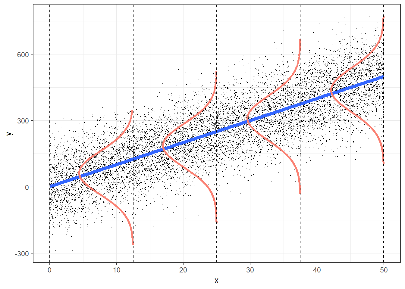
Figure 3.4: Ordinary least squares assumptions
The four main assumptions can be remembered using the acronym ‘LINE’:
L: there is a linear or straightline relationship between the mean response (Y) and the explanatory variable (X). In the figure above, the mean value for Y at each level of X falls on the blue regression line.
I: the errors are independent — there’s no connection between how far any two points lie from the regression line. This is usually more of an issue in time series data (i.e. where data is collected from the same entity over time, e.g. a stock price) than cross-sectional data (where data is collected from many entities a single point in time, e.g. exam marks for a group of students).
N: the dependent variable is normally distributed at each level of X. At each level of X, the values for Y follow a normal or ‘bell-shaped’ distribution as shown in red in the figure above.
E: there is equal variance (or ‘homoscedasticity’) - the variance or ‘spread’ of the responses is equal for all levels of X. The spread in the Y’s for each level of X is the same, as shown above.
A more detailed explanation of these assumptions is provided here by Laerd.
The p-value is the probability of getting a value as extreme or more extreme than the one observed in your sample, under the assumption that the null hypothesis is true.↩