Chapter 5 One mean
This set of tests deals with a single mean. They tell us whether, based on our sample, we have reason to believe that the mean of the underlying population differs from an some specific level (the ‘null hypothesis’).
In some cases we might have two samples with paired observations (e.g. an athlete’s average running speed before and after a new training technique is used). In this case we take the difference between the paired observations (the change in each athlete’s running speed) and treat this as a single measurement. We then assess whether, based on the mean of these differences in our sample, we have reason to believe that the ‘true’ mean differs from a specified level (e.g. zero, representing no change in running speed).
The one sample and paired sample cases are addressed in turn, below.
5.1 One sample
5.1.1 One-sample t-test
A one-sample t-test (or one-sample Student’s t-test) is used to determine whether a sample could have come from a population with a specified mean. This population mean is not always known and may only be theoretical / hypothesized.
For example, say we take a sample of pupils who have been taught using a new teaching method. These pupils receive an average score of 70% in an end-of-year test, while the average score for all pupils nationally is 60%. We want to know how often we are likely to see a sample average of 70% (or more extreme) if the ‘true’ average for pupils receiving the new teaching method was 60%, i.e. if there was no difference from the national average.
Student’s t-test:
In R, we can run a one-sample Student’s t-test using the built-in t.test(). The documentation for this test can be found here.
Equivalent linear model:
The one-sample t-test is the same as a linear model containing a dependent variable, \(y\), and a constant only. That is, a model with the form:
\(y = \beta_0 \qquad H_0: \beta_0 = 0\)
This is the same as the equation \(y = \beta_0 + \beta_1 \cdot x\) that was shown earlier (Chapter 3), but having dropped the last term. This is shown graphically below. Note that this is the same as a linear regression in which all values of \(x\) are treated as zero:
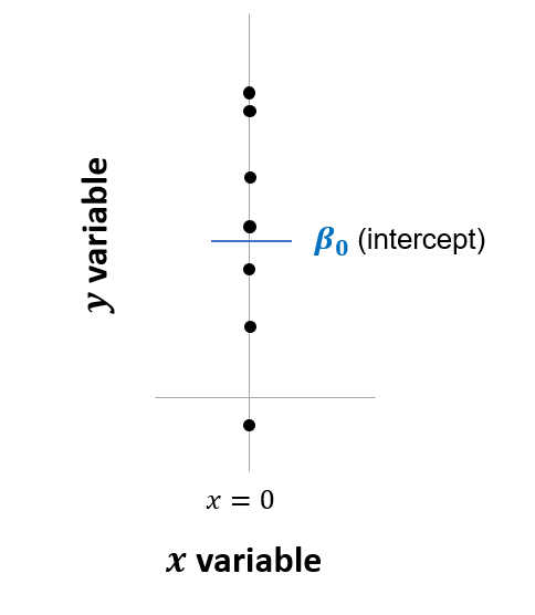
Figure 5.1: Linear model equivalent to one-sample t-test
The estimated intercept (\(\beta_0\)) is simply the average of all the values in our sample. The linear regression returns the t-statistic and p-value based on the null hypothesis that the true average is equal to zero (i.e. \(\beta_0 = 0\)).
Comparison:
Here is how you would run the t-test and equivalent linear model in R:
# t-test (built-in test)
t.test(y, mu = 0, alternative = 'two.sided')

# Linear model
lm <- lm(y ~ 1)
  lm %>% summary() %>% print(digits = 5) # show summary output
  confint(lm) # show confidence intervals
The output of this code, including the 95 percent confidence intervals, is shown in the table below. The outputs are exactly the same!
| Test | mean / intercept | t | p.value | conf.low | conf.high |
|---|---|---|---|---|---|
| t.test | 0.3 | 1.0607 | 0.294 | -0.2684 | 0.8684 |
| lm | 0.3 | 1.0607 | 0.294 | -0.2684 | 0.8684 |
Based on the p-value above, despite having a sample average of 0.3 we would not reject the null hypothesis that the true or population average was zero (at the 0.05 level of significance).
Testing a null hypothesis other than zero:
By default, the t-test has a null hypothesis is that the sample comes from a population with a mean of zero. This was written as \(H_0: \beta_0 = 0\) above. What if we want to use a different null hypothesis? For example, to how likely it is that our sample y came from a population with a mean of 0.1?
This can be done by specifying the null hypothesis in the built-in t-test (in this case using the argument mu = 0.1) or, in the linear model, by first subtracting this amount from the dependent variable (using y - 0.1 as the dependent variable).
The code is as follows:
# t-test (built-in test)
t.test(y, mu = 0.1, alternative = 'two.sided')

# Linear model
lm((y - 0.1) ~ 1) %>%
  summary() %>% print(digits = 5) # show summary output
The two tests above give identical t statistics and p-values.
5.1.2 Wilcoxen signed-rank
What if we cannot assume that our population is normally distributed? Here we need to use a non-parametric version of the t-test.
Wilcoxen signed-rank test:
In this case we could use the Wilcoxon signed-rank test, which is the non-parametric version of the t-test. Specifically, we use the one-sample Wilcoxon signed-rank test. This is used to determine whether the median of the sample is equal to a theoretical value, such as zero, under the assumption that the data is symmetrically distributed.
The Wilcoxon signed-rank test is very similar to the linear model described above, but using the signed ranks of \(y\) instead of \(y\) itself. The concept of signed ranks was explained in section 2.2.
It is implemented in R using the wilcox.test, as shown below.
Equivalent linear model:
In this case the equivalent linear model is:
\(signed\_rank(y) = \beta_0 \qquad H_0: \beta_0 = 0\)
Lindeløv shows that the linear model will be a good approximation of the Wilcoxon signed-rank test when the sample size is larger than 14 and almost perfect when the sample size is larger than 50.
Comparison:
The code below is for the wilcox.test in R and the equivalent linear model using signed ranks:
# Wilcox test (built-in)
wilcox.test(y)

# Equivalent linear model
lm <- lm(signed_rank(y) ~ 1)
lm %>% summary() %>% print(digits = 8) # show summary output| Test | mean / intercept | p.value |
|---|---|---|
| wilcox.test | 0.3693 | |
| lm (signed ranks) | 3.74 | 0.3721 |
The two tests give similar (though not quite identical) p-values.
5.2 Paired samples
5.2.1 Paired-sample t-test
A paired-sample t-test (sometime called a dependent-sample t-test) is used to compare two population means where you have two samples, in which observations in one sample can be paired with observations in the other sample.
Common applications of the paired-sample t-test include controlled studies or repeated-measures designs. Examples of when you might use this test include:
- Before and after observations on the same subjects (e.g. students’ test results before and after taking a course).
- A comparison of two different treatments, where where the treatments are applied to the same subjects (e.g. athletes’ ability to lift weights following two different warm-up routines).
- A comparison of two different measurements, where where the measurements are applied to the same subjects (e.g. blood pressure measured using two types of machines).
Paired-sample t-test / dependent-sample t-test:
The paired-sample t-test determines whether the average difference between two sets of observations is zero. To run this in R, we use the same Student’s t-test as above, but now include both variables as arguments and specify that we have paired observations (using the argument paired = TRUE).
Equivalent linear model:
The equivalent linear model is the difference between the two observations regressed against a constant:
\(y_2 - y_1 = \beta_0 \qquad H_0: \beta_0 = 0\)
Comparison:
We can compare the t-test and linear model using our sample data (section 2.1) as an example. Recall that y had a mean of 0.3, and y2 had a mean of 0.5.
The code and the outputs are shown below. Again, the linear model gives exactly the same results as the t-test!
# t-test (built-in test)
t.test(y2,y, paired = TRUE, mu = 0, alternative = 'two.sided')

# Equivalent linear model
lm <- lm(y2 - y ~ 1)
  lm %>% summary() %>% print(digits = 8)
confint(lm)| Test | mean of diff / intercept | t | p.value | conf.low | conf.high |
|---|---|---|---|---|---|
| t.test | 0.2 | 0.5264 | 0.601 | -0.5635 | 0.9635 |
| lm | 0.2 | 0.5264 | 0.601 | -0.5635 | 0.9635 |
This shows us that the difference in averages between y and y2 is 0.2, as would be expected, but that this difference is not statistically significantly difference from zero (p = 0.601) at the 0.05 level of significance.
5.2.2 Wilcoxen matched pairs
If the necessary assumptions do not hold for a paired-sample t-test - such as normally distributed data - we can use the non-parametric counterpart. This is the Wilcoxen matched pairs test. The only difference from the Wilcoxon signed-rank test is that it’s testing the signed ranks of the pairwise \(y−x\) differences.
This is used to test the null hypothesis that the median of the differences in our paired observations are zero. An assumption is that the values of the pairwise differences are symmetrically distributed, as explained by Laerd.
For this we use the built-in wilcox.test in R, including both variables and specifying that we have paired observations (the argument paired = TRUE).
The equivalent linear model is exactly the same above but using signed rank of the difference between observations, i.e.:
\(signed\_rank(y_2 - y_1) = \beta_0 \qquad H_0: \beta_0 = 0\)
A comparison of the outputs is shown below. The p-values are almost identical. The t-test has also been included, this time using signed ranks, to show that this is the same as the linear model.
#  Wilcox test (built-in test)
wilcox.test(y2,y, paired = TRUE, mu = 0, alternative = 'two.sided')

# Equivalent linear model
lm <- lm(signed_rank(y2 - y) ~ 1)
  lm %>% summary() %>% print(digits = 8)

# t-test using signed ranks (built-in test)
t.test(signed_rank(y2-y), mu = 0, alternative = 'two.sided')| Test | mean / intercept | p.value |
|---|---|---|
| wilcox.test | 0.8243 | |
| lm (signed ranks) | 0.94 | 0.8232 |
| t.test (signed ranks) | 0.94 | 0.8232 |
Based on the results above, we would not reject the null hypothesis that the median change between y and y2 was zero (p = 0.8232), at the 0.05 level of significance.